Code
# Load packages
library(sf)
library(dplyr)
library(httr2)
library(stringr)
library(tidyverse)
library(leaflet)
library(grid)New York City’s landscape is more than towers and traffic, it is also home to nearly one million trees that form the city’s “urban forest.” These quiet giants work around the clock to keep the city livable:
With this project, I take on the role of a tree detective, using public data to understand where NYC’s canopy thrives and where it needs the most care. The goal is to build evidence for future investments that make District 4’s trees more resilient to climate change.
This project follows the analytical workflow used by urban-data professionals and city agencies:
Through this process, we contribute to a broader conversation: how can New York ensure that the benefits of its trees are equitably shared among all neighborhoods?
# Load packages
library(sf)
library(dplyr)
library(httr2)
library(stringr)
library(tidyverse)
library(leaflet)
library(grid)Source: NYC Department of City Planning Council Districts (nycc_25c.zip).
These boundaries define New York’s 51 City Council Districts. Understanding tree distribution by district is essential for equitable maintenance funding and local environmental planning.
The code in chunk download_boundaries below:
(data/mp03/) if it doesn’t existsf::st_read()Each row of the resulting object districts represents a Council District polygon with unique ID, geometry, and shape measurements.
# Create a local folder (data/mp03/) if it does not exist
download_nyc_districts <- function() {
  if(!dir.exists(file.path("data", "mp03"))){
    dir.create(file.path("data", "mp03"), showWarnings=FALSE, recursive=TRUE)
  }

  ZIP_FILENAME <- file.path("data", "mp03", "nycc_districts.zip")
  URL <- "https://s-media.nyc.gov/agencies/dcp/assets/files/zip/data-tools/bytes/city-council/nycc_25c.zip"

# Download the ZIP file only if it’s not already saved locally

  if(!file.exists(ZIP_FILENAME)){
    download.file(URL, destfile=ZIP_FILENAME, mode = "wb", quiet = TRUE)
  }

  UNZIP_DIR <- file.path("data", "mp03", "unzipped")
  SHP_FILE  <- file.path(UNZIP_DIR, "nycc_25c", "nycc.shp")

# Unzip only if the shapefile hasnot been extracted yet
  if(!file.exists(SHP_FILE)){
    if(!dir.exists(UNZIP_DIR)){
      dir.create(UNZIP_DIR, showWarnings = FALSE, recursive = TRUE)
    }
    unzip(ZIP_FILENAME, exdir=UNZIP_DIR)
  }

# Read the shapefile quietly, convert to NYC’s local projection (EPSG:2263),
# simplify boundaries to speed up plotting, and then reproject to WGS84 for mapping
  districts <- sf::st_read(SHP_FILE, quiet = TRUE) |>
    sf::st_transform(2263) |>
    dplyr::mutate(geometry = sf::st_simplify(geometry, dTolerance = 50)) |>
    sf::st_transform(4326)

  return(districts)
}

# Run the function and save the result as 'districts'
districts <- download_nyc_districts()Source: NYC Open Data, Forestry Tree Points (hn5i-inap) via API (SODA2).
The Parks Department maintains a record of nearly 900,000 trees, including species, condition, and size.
These data, provided through the Socrata (SODA2) API, allow us to map trees to their council districts and assess canopy health citywide.
The function in chunk tree_dataset downloads the data responsibly:
$limit and $offset parametershttr2’s req_url_query() + req_retry() + req_perform() pattern for reliabilitydata/mp03/ to prevent repeated requestsbind_rows() into a single sf object called treesEach record in trees includes geographic coordinates and key attributes like species (genusspecies), diameter (dbh), and condition (tpcondition).
# Create a local folder (data/mp03/) if it does not  exist
download_nyc_trees <- function() {
  if(!dir.exists(file.path("data", "mp03"))){
    dir.create(file.path("data", "mp03"), showWarnings=FALSE, recursive=TRUE)
  }

  LIMIT <- 5000L  # No. of records per API call
  OFFSET <- 0L # Starting point for each batch
  ALL_TREES <- list() # List to store downloaded batches
  END_OF_DATA <- FALSE

# Loop through the dataset in batches using $limit and $offset

  while(!END_OF_DATA){
    TREE_FILENAME <- file.path("data", "mp03", paste0("nyc_trees_", OFFSET, ".geojson"))

# Download the GeoJSON file only if it’s not already saved locally

    if(!file.exists(TREE_FILENAME)){
      request("https://data.cityofnewyork.us/resource/hn5i-inap.geojson") |>
        req_url_query(`$limit` = LIMIT, `$offset` = OFFSET) |>
        req_retry(max_tries=5) |>
        req_perform(path = TREE_FILENAME)
    }

# Read the downloaded GeoJSON file quietly
    tree_data <- sf::st_read(TREE_FILENAME, quiet = TRUE)

# If the file is empty, stop the loop
# Convert date columns to character format for consistency
    if(nrow(tree_data) == 0){
      END_OF_DATA <- TRUE
    } else {
      tree_data$planteddate <- as.character(tree_data$planteddate)
      ALL_TREES <- c(ALL_TREES, list(tree_data))

 # If fewer than LIMIT rows were returned, we’ve reached the end
# Otherwise, move to the next batch
      if(nrow(tree_data) < LIMIT){
        END_OF_DATA <- TRUE
      } else {
        OFFSET <- OFFSET + LIMIT
      }
    }
  }

 # Combine all downloaded batches into one sf object
  trees <- dplyr::bind_rows(ALL_TREES)
  return(trees)
}

# Run the function and store the combined data as 'trees'
trees <- download_nyc_trees()To prepare for analysis, variable names were standardized and key fields checked for missing or inconsistent entries. Both datasets were lightly cleaned so they are consistent, easy to read, and ready for mapping.
Columns such as CounDist, Shape_Leng, and Shape_Area were renamed to clearer, more descriptive names.
This makes the data easier to interpret while keeping all original information intact.
districts <- districts |>
  rename(council_district = CounDist,
         shape_length = Shape_Leng,
shape_area = Shape_Area)To prepare the tree dataset, columns were renamed to intuitive names, and missing or unclear values were standardized.
Columns such as tpcondition, riskrating, and dbh were renamed to tree_condition, risk_rating, and tree_diameter.
Missing entries were labeled as "Unknown" or "Not Rated" to keep summaries easy to read.
# Clean the column names
trees <- trees |>
  rename(
    tree_condition = tpcondition,
    stump_diameter = stumpdiameter,
    risk_rating_date = riskratingdate,
    risk_rating = riskrating,
    object_id = objectid,
    global_id = globalid,
    tree_structure = tpstructure,
    planting_space_id = plantingspaceglobalid,
    created_date = createddate,
    tree_diameter = dbh,
    planted_date = planteddate,
    updated_date = updateddate,
    genus_species = genusspecies
  )

# Handle NA values
trees <- trees |>
  mutate(
    tree_condition = ifelse(is.na(tree_condition), "Unknown", tree_condition),
    risk_rating = ifelse(is.na(risk_rating), "Not Rated", risk_rating),
    tree_diameter = as.numeric(tree_diameter),
    tree_diameter = ifelse(is.na(tree_diameter), median(tree_diameter, na.rm = TRUE), tree_diameter))
After renaming and standardizing the dataset, it is important to confirm that all key fields are complete and reliable.
A quick summary below checks for missing values in tree condition, risk rating, and diameter, helping ensure that future visualizations and comparisons are based on accurate and consistent information.
# Check for missing values in key columns to confirm data completeness
na_tree_condition <- sum(is.na(trees$tree_condition))
na_risk_rating    <- sum(is.na(trees$risk_rating))
na_tree_diameter  <- sum(is.na(trees$tree_diameter))
c(na_tree_condition = na_tree_condition,
  na_risk_rating    = na_risk_rating,
  na_tree_diameter  = na_tree_diameter)
na_tree_condition na_risk_rating na_tree_diameter
0 0 0 All three fields showed zero missing values, confirming that the cleaned dataset is complete and ready for analysis.
Geospatial visualization provides an effective way to assess the scale, condition, and spatial distribution of New York City’s tree canopy.
The following analyses combine point-level tree data with council district boundaries to identify areas of strength and vulnerability across the city’s “urban forest.”
A citywide map overlays individual tree points on the 51 City Council District boundaries to illustrate the extent of canopy coverage.
The visualization reveals broad spatial patterns—dense concentrations in Central Park, Prospect Park, and residential neighborhoods, contrasted with sparser coverage in commercial and industrial zones.
This view highlights both the magnitude of the dataset and the uneven distribution of trees across the five boroughs.
# Plot all tree points over NYC Council District boundaries
ggplot() +
  geom_sf(data = districts, aes(fill = "Council Districts"), color = "blue", alpha = 0.3) +
  geom_sf(data = trees, aes(color = "Tree Locations"), size = 0.1, alpha = 0.02) +
  scale_fill_manual(
    name = "Boundaries",
    values = c("Council Districts" = "lightblue"),
    guide = guide_legend(override.aes = list(alpha = 0.5))
  ) +
  scale_color_manual(
    name = "Trees",
    values = c("Tree Locations" = "darkgreen")
  ) +
  labs(title = "NYC Trees by Council District",
       subtitle = paste(scales::comma(nrow(trees)), "trees across New York City")) +
  theme_minimal() +
  theme(legend.position = "bottom")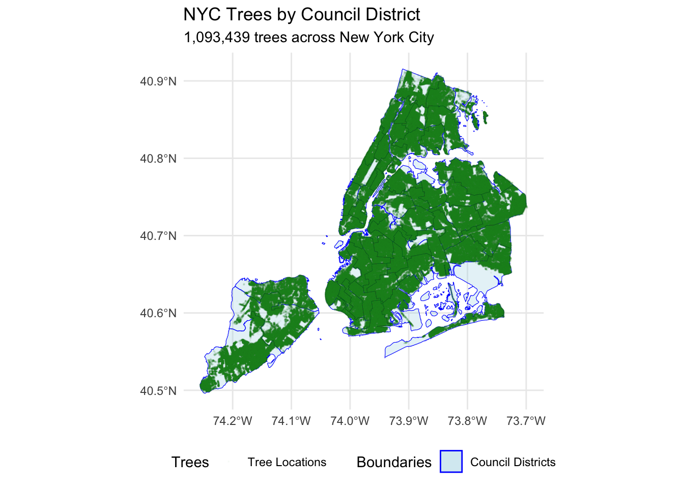
An interactive Leaflet map summarizes tree density (trees per km²) at the borough level. Each polygon is shaded by canopy density, allowing users to compare borough-level coverage at a glance.
This view confirms that while Queens and Brooklyn account for the largest total number of trees, Manhattan exhibits the highest density relative to land area—reflecting smaller geographic size and concentrated green corridors.
all_trees <- trees

# every district has a borough label (no NAs), and keeping only labeled rows
districts_named <- districts |>
  dplyr::mutate(
    borough = dplyr::case_when(
      council_district >=  1 & council_district <= 10 ~ "Manhattan",
      council_district >= 11 & council_district <= 18 ~ "Bronx",
      council_district >= 19 & council_district <= 32 ~ "Queens",
      council_district >= 33 & council_district <= 48 ~ "Brooklyn",
      council_district >= 49 & council_district <= 51 ~ "Staten Island",
      TRUE ~ NA_character_
    )
  ) |>
  dplyr::filter(!is.na(borough))

# Building one multipolygon per borough
borough_outline <- districts_named |>
  sf::st_make_valid() |>
  dplyr::group_by(borough) |>
  dplyr::summarise(.groups = "drop") |>
  sf::st_cast("MULTIPOLYGON", warn = FALSE)

# Join trees to districts (points within polygons) and count per district
trees_with_districts <- sf::st_join(trees, districts_named, join = sf::st_within)

trees_per_district <- trees_with_districts |>
  sf::st_drop_geometry() |>
  dplyr::count(council_district, name = "tree_count")

# Accurate district area (ft^2 -> m^2 -> km^2) using EPSG:2263
districts_area <- districts_named |>
  sf::st_transform(2263) |>
  dplyr::mutate(area_m2 = as.numeric(sf::st_area(geometry)) * (0.3048006096^2)) |>
  sf::st_drop_geometry() |>
  dplyr::transmute(council_district, area_km2 = area_m2 / 1e6)

# Merge counts + area and compute density
districts_density <- districts_named |>
  dplyr::left_join(trees_per_district, by = "council_district") |>
  dplyr::left_join(districts_area,      by = "council_district") |>
  dplyr::mutate(
    tree_count = ifelse(is.na(tree_count), 0L, tree_count),
    density    = tree_count / area_km2
  )

# Popups + palette
pal <- leaflet::colorNumeric("YlGnBu", domain = districts_density$density)

districts_density$popup <- paste0(
  "<b>Borough:</b> ", districts_density$borough, "<br>",
  "<b>District:</b> ", districts_density$council_district, "<br>",
  "<b>Trees:</b> ", format(districts_density$tree_count, big.mark = ","), "<br>",
  "<b>Area:</b> ", round(districts_density$area_km2, 1), " km²<br>",
  "<b>Density:</b> ", round(districts_density$density, 1), " trees/km²"
)

# Leaflet map (NYC-only viewport)
leaflet::leaflet(districts_density) |>
  leaflet::addProviderTiles(leaflet::providers$CartoDB.Positron) |>
  leaflet::addPolygons(
    fillColor    = ~pal(density),
    color        = "white",
    weight       = 1,
    fillOpacity  = 0.85,
    popup        = ~popup
  ) |>
  leaflet::addPolylines(
    data   = borough_outline,
    color  = "black",
    weight = 1,  # Thinner boundary lines
    opacity= 0.6
  ) |>
  leaflet::addLegend(
    position = "bottomright",
    pal      = pal,
    values   = ~density,
    title    = "Tree Density (trees/km²)",
    opacity  = 1
  ) |>
leaflet::setView(lng = -73.94, lat = 40.70, zoom = 11) # Zoomed in on NYCThis section analyzes how trees are distributed across New York City’s 51 Council Districts.
By integrating tree point data with district boundaries, it quantifies canopy coverage, density, and condition, highlighting both areas of strength and those that may need more investment.
Key measures include total tree count, canopy density, and tree health. The analysis also explores species composition in Manhattan and concludes with a hyperlocal example near Baruch College.
Identifying which districts host the most trees helps reveal where canopy coverage is concentrated and where new planting might be needed.
# count of trees per district
trees_per_district <- trees_with_districts |>
  count(council_district, name = "tree_count") |>
arrange(desc(tree_count))Finding: Council District 51 has the most trees with 70925 trees.
Tree density measures how concentrated trees are relative to land area, providing a clearer picture of canopy coverage beyond simple counts.
# Calculate tree density per district using geometric area_km2
tree_density <- districts_density |>
  sf::st_drop_geometry() |>
  select(council_district, tree_count, area_km2) |>
  mutate(tree_density = tree_count / area_km2) |>
arrange(desc(tree_density))Finding: District 7 shows the highest tree density, meaning it supports the most trees per unit of land.
Examining tree condition across districts helps pinpoint areas with higher rates of tree loss or stress, signaling where maintenance or replacement efforts should be prioritized
# Count dead trees in each district
dead_trees <- trees_with_districts |>
  group_by(council_district) |>
  summarise(
    total_trees = n(),
    dead_trees = sum(tree_condition == "Dead", na.rm = TRUE),
    dead_fraction = dead_trees / total_trees
  ) |>
arrange(desc(dead_fraction))Finding: District 32 has the highest share of dead trees 14.2%, suggesting greater vulnerability or lower maintenance investment in that area.
Analyzing which species dominate Manhattan’s canopy reveals patterns of biodiversity and guides future planting for ecological resilience.
# Add borough column using case_when
trees_with_boroughs <- trees_with_districts |>
  mutate(
    borough = case_when(
      council_district <= 10 ~ "Manhattan",
      council_district <= 18 ~ "Bronx",
      council_district <= 32 ~ "Queens",
      council_district <= 48 ~ "Brooklyn",
      council_district <= 51 ~ "Staten Island"
    )
  )

# Find most common tree species in Manhattan
manhattan_trees <- trees_with_boroughs |>
  filter(borough == "Manhattan") |>
  count( genus_species, name = "count") |>
arrange(desc(count))Finding: The species Gleditsia triacanthos var. inermis - Thornless honeylocust is the most common in Manhattan, with 17307 recorded trees.
A hyperlocal analysis reveals the tree closest to Baruch College.
# create  function
new_st_point <- function(lat, lon, ...){
    st_sfc(st_point(c(lon, lat))) |>
      st_set_crs("WGS84")
}

# create Baruch point and find closest tree
baruch_point <- new_st_point(40.7405, -73.9832)

twd_for_baruch <- sf::st_join(trees, districts, join = st_within)
closest_tree <- twd_for_baruch |>
  dplyr::mutate(distance_m = units::set_units(sf::st_distance(geometry, baruch_point), "m")) |>
  dplyr::arrange(distance_m) |>
  dplyr::slice(1)

# coords
closest_tree_coords <- sf::st_coordinates(sf::st_centroid(closest_tree$geometry))
baruch_coords <- sf::st_coordinates(baruch_point)
species <- ifelse(is.na(closest_tree$genus_species), "Unknown", closest_tree$genus_species)

dist_m  <- round(as.numeric(closest_tree$distance_m), 1)

# an interactive leaflet map showing tree density by borough

leaflet() |>
  addTiles() |>
  setView(lng = baruch_coords[1], lat = baruch_coords[2], zoom = 19) |>
  addCircleMarkers(
    lng = closest_tree_coords[1],
    lat = closest_tree_coords[2],
    radius = 8,
    color = "red",
    fillColor = "red",
    fillOpacity = 0.8,
    popup = paste0("Closest Tree:<br><b>", species, "</b><br>Distance: ", dist_m, " meters")
  ) |>
  addMarkers(
    lng = baruch_coords[1],
    lat = baruch_coords[2],
    popup = "<b>Baruch College</b>"
)This chunk computes District 4 metrics, defines project scope and budget, and prepares data for the zoomed-in vulnerability map. The code below calculates vulnerability ratios, sets project parameters, and isolates District 4 tree data for visualization.
Code and analysis for flood vulnerability assessment are shown below.
Skip to policy proposal below
# Classify species as flood-vulnerable or resilient; summarize by district
vulnerable_species <- c("Acer platanoides", "Platanus x acerifolia", "Pyrus calleryana",
                        "Ginkgo biloba", "Quercus palustris")
resilient_species  <- c("Quercus bicolor", "Taxodium distichum", "Betula nigra",
                        "Liquidambar styraciflua", "Nyssa sylvatica")

species_vulnerability <- trees_with_districts |>
  mutate(
    is_vulnerable = str_detect(genus_species, paste(vulnerable_species, collapse = "|")),
    is_resilient  = str_detect(genus_species, paste(resilient_species,  collapse = "|"))
  ) |>
  group_by(council_district) |>
  summarise(
    total_trees         = n(),
    vulnerable_count    = sum(is_vulnerable, na.rm = TRUE),
    resilient_count     = sum(is_resilient,  na.rm = TRUE),
    vulnerability_ratio = vulnerable_count / total_trees,
    resilience_ratio    = resilient_count  / total_trees,
    .groups = "drop"
  ) |>
  arrange(desc(vulnerability_ratio))

#   District 4 and three peer districts
target_district      <- 4
comparison_districts <- c(2, 6, 39)

district_analysis <- species_vulnerability |>
  filter(council_district %in% c(target_district, comparison_districts)) |>
mutate(council_district = factor(council_district, levels = c(2,4,6,39)))# Create vulnerability comparison bar chart
comparison_data <- district_analysis |>
select(council_district, vulnerability_ratio, resilience_ratio) |>
pivot_longer(cols = c(vulnerability_ratio, resilience_ratio),
names_to = "metric", values_to = "ratio") |>
mutate(metric_type = ifelse(metric == "vulnerability_ratio", "Vulnerable", "Resilient"))
vulnerability_chart <- ggplot(
comparison_data,
aes(x = factor(council_district), y = ratio, fill = metric_type)
) +
geom_col(position = "dodge", alpha = 0.85, width = 0.7) +
geom_text(
aes(label = paste0(round(ratio * 100, 1), "%")),
position = position_dodge(width = 0.7),
vjust = -0.5, size = 3.5, fontface = "bold"
) +
scale_y_continuous(labels = scales::percent, limits = c(0, 0.35)) +
scale_fill_manual(values = c("Vulnerable" = "#D32F2F", "Resilient" = "#388E3C")) +
labs(
title = "Flood-Vulnerable vs. Resilient Tree Species by Council District",
subtitle = "District 4 shows both high vulnerability and opportunity for improvement",
x = "Council District",
y = "Percentage of Tree Population",
fill = "Species Type"
) +
theme_minimal(base_size = 14) +
theme(
legend.position = "top",
plot.title = element_text(face = "bold", hjust = 0.5),
plot.subtitle = element_text(hjust = 0.5, color = "gray40")
)This chunk computes District 4 metrics, defines project scope and budget, and prepares data for the zoomed-in vulnerability map.
The code below calculates vulnerability ratios, sets project parameters, and isolates District 4 tree data for visualization.
# Calculate District 4 metrics
district4_metrics <- species_vulnerability |>
  filter(council_district == target_district)

district4_vulnerability <- round(district4_metrics$vulnerability_ratio * 100, 1)
avg_comparison_vulnerability <- round(
  mean(
    district_analysis$vulnerability_ratio[
      district_analysis$council_district != target_district
    ]
  ) * 100,
  1
)

# Define scope and budget
proposed_replacements   <- round(district4_metrics$vulnerable_count * 0.3)
new_resilient_plantings <- 150
total_interventions     <- proposed_replacements + new_resilient_plantings
estimated_budget        <- total_interventions * 2000

# Prepare map data (District 4 boundary + trees with climate categories)
d4_boundary <- districts |> filter(council_district == target_district)

d4_trees <- trees_with_districts |>
  filter(council_district == target_district) |>
  mutate(
    vulnerability_status = case_when(
      str_detect(genus_species, paste(vulnerable_species, collapse = "|")) ~ "Vulnerable",
      str_detect(genus_species, paste(resilient_species,  collapse = "|")) ~ "Resilient",
      TRUE ~ "Other"
    )
  )

# Bounding box for  zoom
bb <- st_bbox(d4_boundary)To: NYC Department of Parks & Recreation (DPR); Mayor’s Office of Climate & Environmental Justice
From: Office of the Council Member, District 4
Date: December 13, 2025
Subject: Climate-Resilient Tree Initiative
Across New York City, nearly 900,000 street and park trees create an urban forest that cools neighborhoods, cleans the air, and manages stormwater. Yet the city’s canopy faces growing stress from flooding and extreme rainfall events.
District 4 was selected for this initiative given its extensive East River waterfront and concentration of flood-vulnerable infrastructure, including hospitals, schools, and major transit corridors along the 23rd–34th Street corridor.
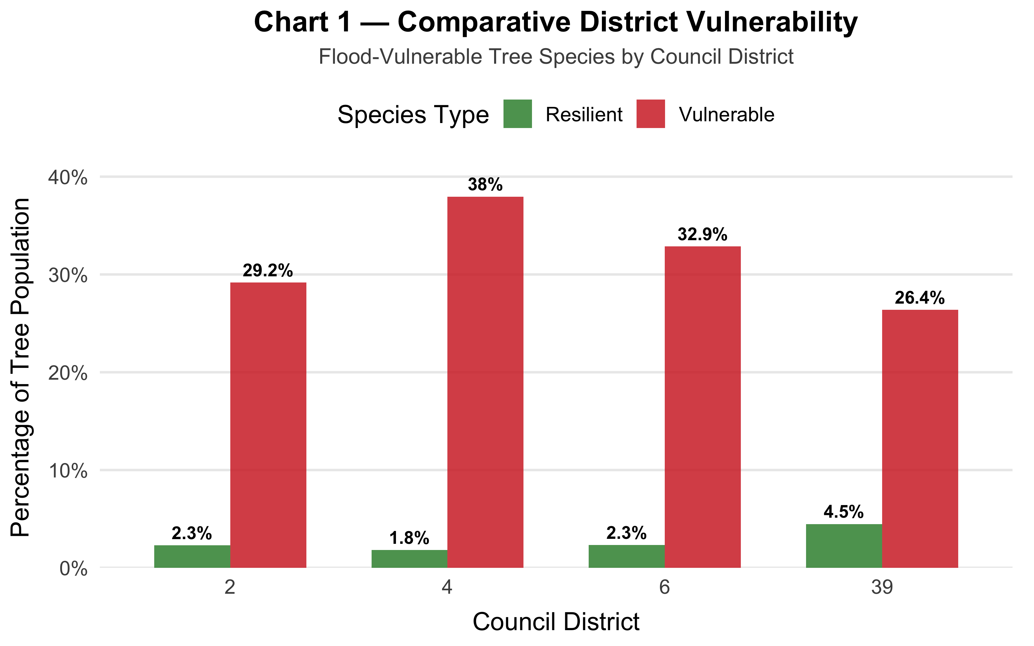
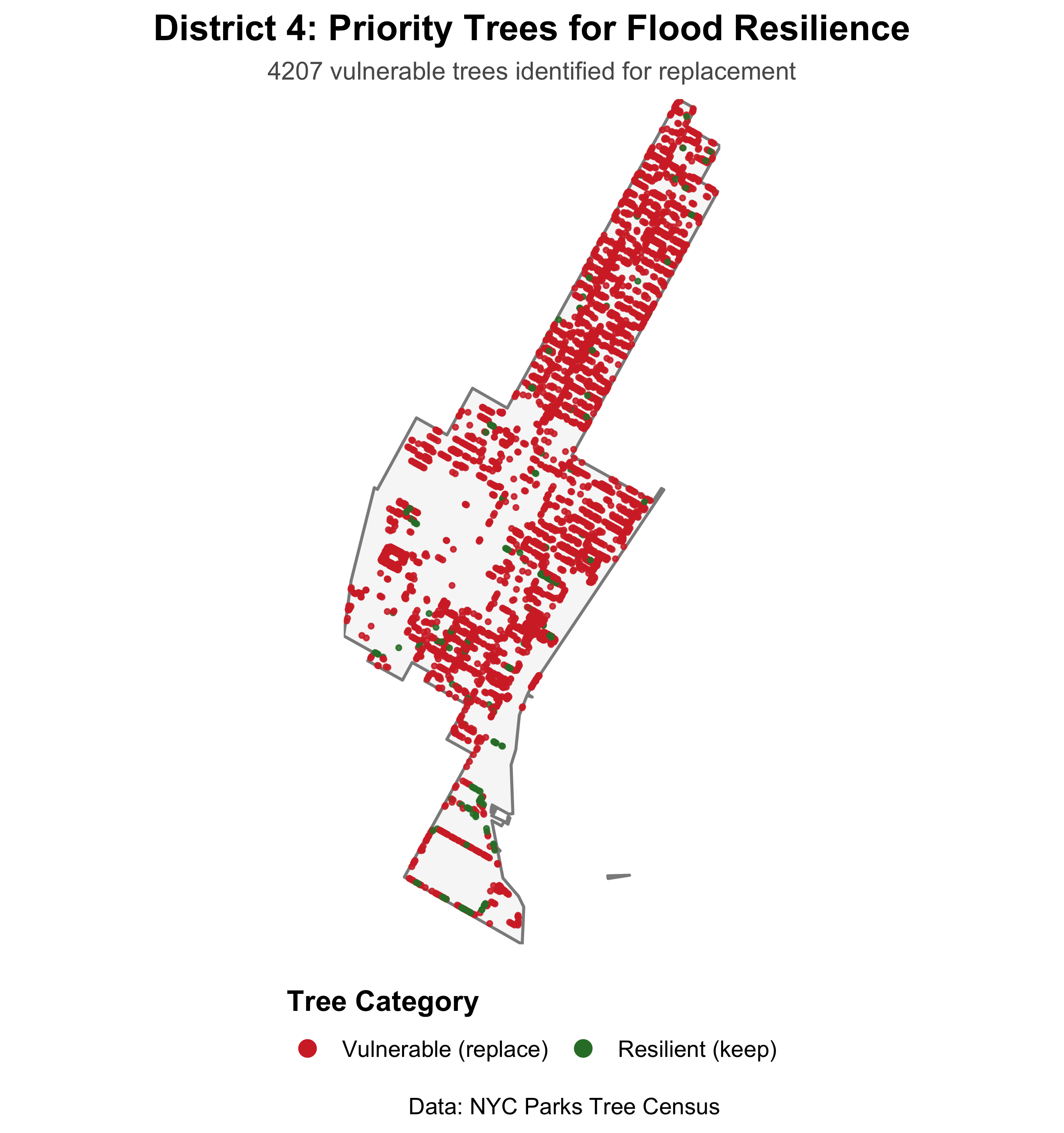
Our analysis of the NYC Parks Tree Census finds that District 4 has a higher share of flood-vulnerable tree species (38%) than neighboring Manhattan districts (29.5% average). These at-risk trees cluster along East 23rd–34th Streets, Lexington Avenue, and the East River Esplanade, corridors that also serve schools, senior centers, and major transit routes (see Chart 1 below for district comparison).
To strengthen canopy resilience, the Council Office proposes the District 4 Climate-Resilient Canopy Initiative, a data-driven program to replace vulnerable trees and expand flood-tolerant plantings in priority locations (see Map 1 below).
The project would remove approximately 1262 high-risk trees (including flood-sensitive species like Norway Maple and London Planetree) and install 150 new flood-tolerant species such as Swamp White Oak, Bald Cypress, and River Birch.
Altogether, these actions total 1412 interventions, with an estimated budget of $2,824,000 covering removal, planting, soil improvement, and stewardship support.
This initiative aligns directly with New York City’s 2023 Climate Resiliency Plan and the Parks Department’s Urban Canopy Strategy, reducing reliance on flood-intolerant species and lowering long-term emergency removal costs. Beyond resilience, it advances multiple co-benefits: cooler summer streets, cleaner air, and stronger neighborhood engagement through resident care guides and stewardship sign-ups.
By acting now, DPR can safeguard District 4’s canopy before recurring storms cause irreversible losses. This project illustrates how local data can guide equitable, cost-effective adaptation, providing a replicable model for other flood-prone districts citywide.
Chart 1 — Comparative District Vulnerability
vulnerability_chart +
  labs(
    title = "Chart 1 — Comparative District Vulnerability",
    subtitle = "Flood-Vulnerable Tree Species by Council District"
  ) +
  scale_y_continuous(
    labels = scales::percent_format(accuracy = 1),
    limits = c(0, NA),
    expand = expansion(mult = c(0, .08))
  ) +
  theme(
    plot.title         = element_text(face = "bold", size = 16, margin = margin(b = 6)),
    plot.subtitle      = element_text(size = 12, colour = "gray30", margin = margin(b = 10)),
    axis.title.x       = element_text(margin = margin(t = 8)),
    axis.title.y       = element_text(margin = margin(r = 8)),
    panel.grid.minor   = element_blank(),
    panel.grid.major.x = element_blank(),
    plot.margin        = margin(t = 6, r = 12, b = 6, l = 6)
  )
Map 1 — District 4 Priority Intervention Areas
# Count for subtitle (brief metric)
vuln_count <- sum(d4_trees$vulnerability_status == "Vulnerable", na.rm = TRUE)

# Filter out "Other" trees to reduce clustering
d4_trees_filtered <- d4_trees |>
  filter(vulnerability_status != "Other")

# ensure legend order is consistent
d4_trees_filtered$vulnerability_status <- factor(
  d4_trees_filtered$vulnerability_status,
  levels = c("Vulnerable", "Resilient")
)

ggplot() +
  # District boundary
  geom_sf(data = d4_boundary, fill = "grey97", color = "grey55", linewidth = 0.6) +

  # Only vulnerable and resilient trees
  geom_sf(
    data = d4_trees_filtered,
    aes(color = vulnerability_status),
    size = 0.7, alpha = 0.85
  ) +

  # Clear, accessible palette + legend labels
  scale_color_manual(
    values = c("Vulnerable" = "#D32F2F", "Resilient" = "#2E7D32"),
    labels = c("Vulnerable (replace)", "Resilient (keep)"),
    name   = "Tree Category"
  ) +

  # Tight zoom to District 4
  coord_sf(
    xlim = c(bb["xmin"], bb["xmax"]),
    ylim = c(bb["ymin"], bb["ymax"]),
    expand = FALSE,
    datum = NA
  ) +

  labs(
    title    = "District 4: Priority Trees for Flood Resilience",
    subtitle = paste0(vuln_count, " vulnerable trees identified for replacement"),
    caption  = "Data: NYC Parks Tree Census"
  ) +

  theme_minimal(base_size = 12) +
  theme(
    legend.position   = "bottom",
    legend.title      = element_text(face = "bold"),
    plot.title        = element_text(face = "bold", size = 15, hjust = 0.5),
    plot.subtitle     = element_text(size = 10.5, hjust = 0.5, colour = "gray35"),
    panel.grid        = element_blank(),
    plot.margin       = margin(t = 6, r = 8, b = 6, l = 8)
  ) +
  guides(
    color = guide_legend(
      override.aes = list(size = 3, alpha = 1),
      title.position = "top",
      nrow = 1
    )
  )
This work ©2025 was initially prepared as a Mini-Project for STA 9750 at Baruch College.
More details about the course can be found at the course site, and full assignment instructions are available under Mini-Project #03.